Table of Contents
1. Introduction
Robotics and autonomous systems increasingly rely on multi-sensor fusion, particularly combining visual data from cameras with precise geometric data from laser rangefinders (LRFs). The 2D LRF, due to its cost-effectiveness and reliability, is a staple in mobile robotics. However, fusing its data with camera imagery necessitates precise knowledge of their relative pose—a problem known as extrinsic calibration. The core challenge addressed in this paper is that the scanning plane of a 2D LRF is invisible to a standard camera, making direct feature correspondence impossible. This work presents a novel, minimal solution using a single observation of a specially designed V-shaped target.
2. Methodology
2.1 Problem Formulation
The goal is to find the rigid transformation $T = \{R, t\}$, where $R$ is a 3x3 rotation matrix and $t$ is a 3x1 translation vector, that maps points from the LRF coordinate frame $L$ to the camera coordinate frame $C$. Without direct correspondences between laser points and pixels, the problem is under-constrained using traditional PnP methods.
2.2 V-Shaped Calibration Target
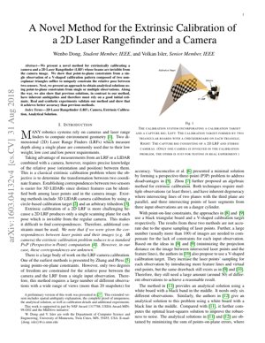
The proposed calibration target, shown in Figure 1 of the PDF, consists of two non-coplanar triangular planes arranged in a V-shape, each adorned with a checkerboard pattern. The checkerboard facilitates accurate pose estimation of each plane relative to the camera. The LRF's scanning plane intersects this V-shape, producing two line segments on the two triangular planes.
2.3 Point-to-Plane Constraints
The core innovation lies in using point-to-plane constraints instead of point-to-point or point-to-line. Each laser point $p^L$ lying on a known plane $\Pi$ in the camera frame must satisfy the plane equation: $n^T (R p^L + t) + d = 0$, where $n$ is the plane's unit normal and $d$ is its distance from the origin. A single observation provides multiple such constraints from the points on both triangles.
3. Analytical Solution
3.1 Mathematical Derivation
The authors demonstrate that the constraints from a single V-shape observation can be formulated into a system of equations. By strategically combining constraints from points on both planes, they eliminate the translation vector $t$ initially, reducing the problem to solving for the rotation $R$ from a quadratic equation. Once $R$ is determined, $t$ can be computed linearly. The solution path avoids the ambiguities present in methods like Vasconcelos et al. [6] and Zhou [7].
3.2 Uniqueness Proof
A significant contribution is the formal proof that the proposed constraints from a single V-shape observation yield a unique solution for the extrinsic parameters, barring degenerate configurations (e.g., the LRF plane being parallel to the intersection line of the two target planes). This eliminates the need for multiple observations or an initial guess, which was a critical flaw in prior art.
4. Experiments and Results
4.1 Synthetic Experiments
Synthetic tests were conducted with varying levels of Gaussian noise added to laser points and image corner detection. The proposed method consistently achieved lower error in rotation and translation estimation compared to baseline methods [5, 6, 7], especially under higher noise conditions, demonstrating its robustness.
4.2 Real-World Experiments
A physical rig with a Hokuyo UTM-30LX LRF and a stereo camera (using only one camera for calibration) was used. The proposed method achieved a mean reprojection error of laser points onto the camera image of approximately 0.3 pixels, outperforming the method by Zhang and Pless [5].
4.3 Comparison with Previous Methods
The paper provides a clear comparative analysis:
- Zhang & Pless [5] (Points-on-Plane): Requires >20 observations, only constrains 2 DoF per observation.
- Vasconcelos et al. [6] (P3P): Requires ≥3 observations, suffers from degeneracy (danger cylinder).
- Proposed Method: Requires only 1 observation (minimal), provides a unique analytical solution, and is immune to the mentioned degeneracies.
5. Technical Analysis & Expert Commentary
Core Insight
This paper isn't just another incremental improvement; it's a fundamental shift in solving a persistent sensor fusion bottleneck. The authors correctly identified that the root of the problem in prior work was inherent ambiguity. Methods like [6] and [7] are essentially trying to solve an ill-posed problem with more data, which is computationally inefficient and unreliable. The key insight is leveraging the 3D geometry of a single, cleverly designed target to inject enough constraints to make the problem well-posed from the get-go. This mirrors the philosophy behind successful minimal solutions in computer vision, such as those for structure-from-motion, where elegance lies in deriving maximum information from minimal data.
Logical Flow
The argument is logically airtight: 1) The invisibility of the laser plane necessitates indirect constraints. 2) Previous methods used constraints that were insufficient per observation, leading to ambiguity. 3) A V-shaped target creates two distinct, non-coplanar intersecting planes with the laser sheet. 4) The point-to-plane constraint from multiple points on these two planes generates a system of equations with a unique solution for the 6-DoF transform. The proof of uniqueness is the linchpin that elevates this from a heuristic to a rigorous method.
Strengths & Flaws
Strengths: The minimal data requirement (single snapshot) is a massive practical advantage for field calibration. The analytical solution guarantees convergence and speed, avoiding the pitfalls of non-linear optimization. The experimental validation is thorough, covering both synthetic noise analysis and real-world performance.
Flaws & Caveats: The method's Achilles' heel is the degenerate configuration. If the laser scanning plane is parallel to the intersection line of the two target planes, the constraints collapse and the solution fails. In practice, this requires careful placement during calibration—a minor but non-trivial operational constraint. Furthermore, the accuracy is contingent on the precise manufacturing and pose estimation of the V-target. Any error in calibrating the target's own geometry (the checkerboard poses) propagates directly into the extrinsic parameters.
Actionable Insights
For practitioners: Adopt this method for rapid, in-field calibration of new robot platforms. Its single-shot nature makes it ideal for verifying calibration after maintenance or impacts. However, always validate with a second, redundant method (e.g., manually measuring key distances) to guard against degenerate setups. For researchers: This work opens the door to investigating other minimal target geometries. Could a tetrahedron or a curved surface provide even more robust constraints? The principle of using high-order geometric primitives (planes over lines/points) for constraint generation is a powerful template for other cross-modal calibration problems, such as radar-camera or thermal-camera fusion, which are gaining traction in autonomous driving research at institutions like Carnegie Mellon's Robotics Institute.
6. Technical Details
6.1 Mathematical Formulation
Let a point in the LRF frame be $p^L = (x^L, y^L, 0)^T$ (since it lies on the LRF's z=0 plane). Its position in the camera frame is $p^C = R p^L + t$. If this point lies on a plane in the camera frame with parameters $\pi = (n^T, d)^T$ where $\|n\|=1$, the point-to-plane distance is zero: $$ n^T (R p^L + t) + d = 0 $$ For $N$ points on the same plane, this forms a system: $$ n^T R P^L + n^T t \cdot \mathbf{1}^T + d \cdot \mathbf{1}^T = \mathbf{0}^T $$ where $P^L$ is a matrix of stacked $p^L$ vectors. The solution strategy involves using points from both planes to eliminate $t$ and solve for $R$ first.
6.2 Calibration Target Geometry
The V-target is defined by two plane equations, $\Pi_1: (n_1, d_1)$ and $\Pi_2: (n_2, d_2)$. The intersection line of these planes is a critical element. The laser scan line $L$ intersects $\Pi_1$ at segment $S_1$ and $\Pi_2$ at segment $S_2$. The 3D coordinates of points on $S_1$ and $S_2$ in the LRF frame are known from the scan, and their corresponding plane identities are known from the geometry of the intersection.
7. Experimental Results & Charts
The paper includes quantitative results best summarized as follows:
Rotation Error (Synthetic)
Proposed Method: ~0.05° - 0.15° across noise levels.
Method [6]: ~0.1° - 0.4°, higher variance.
Method [7]: Often failed or produced >1° error in degenerate-like setups.
Translation Error (Synthetic)
Proposed Method: ~1-3 mm.
Method [5]: >10 mm, required 20+ views to approach similar accuracy.
Real-World Reprojection Error
Proposed Method: 0.3 pixels (mean).
Method [5]: 0.5 - 0.8 pixels.
Lower reprojection error indicates more accurate fusion of laser data into the camera's perspective.
Note: The paper's Figure 1 visually describes the calibration rig and V-target. Subsequent figures likely plot rotation/translation error vs. noise level, demonstrating the proposed method's superior stability.
8. Analysis Framework: Case Example
Scenario: A service robot in a hospital needs its LRF and camera recalibrated after a lens replacement.
- Traditional Method ([5]): Technician must take 20+ images of a checkerboard at different orientations, ensuring the laser line crosses it each time. Process takes 15-20 minutes, prone to human error in view variety.
- Proposed Method: Technician places the V-target in the robot's view. A single snapshot is taken where the laser clearly strikes both wings of the target. Software computes the new calibration in seconds.
Framework Takeaway: The efficiency gain is not linear; it's exponential in terms of operational readiness and reduction in calibration-induced downtime. This framework prioritizes minimal operational friction and deterministic output, which are critical for real-world deployment.
9. Future Applications & Directions
- Dynamic Calibration: Can the principle be extended to perform continuous, online calibration to account for sensor drift due to temperature or vibration, using naturally occurring V-like structures in the environment?
- Multi-Sensor Networks: Calibrating networks of multiple, heterogeneous sensors (e.g., multiple LRFs and cameras on a single autonomous vehicle) using shared target observations.
- Integration with Deep Learning: While analytical methods are robust, a hybrid approach could use a neural network (trained on synthetic data generated using this method's principles) to provide an initial guess for fine-tuning in extremely noisy environments, similar to how DeepLabCut revolutionized pose estimation.
- Standardization: This V-target method has the potential to become a standard benchmark or protocol for 2D LRF-camera calibration, much like the checkerboard is for intrinsic calibration, due to its minimalism and analytical clarity.
10. References
- Thrun, S., et al. (2005). Robotics: Probabilistic Approaches. MIT Press.
- Geiger, A., et al. (2012). Automatic camera and range sensor calibration using a single shot. ICRA.
- Pusztai, Z., & Hajder, L. (2017). Accurate calibration of LiDAR-camera systems using ordinary boxes. ICCV Workshops.
- Lepetit, V., et al. (2009). EPnP: An Accurate O(n) Solution to the PnP Problem. IJCV.
- Zhang, Q., & Pless, R. (2004). Extrinsic calibration of a camera and laser range finder. IROS.
- Vasconcelos, F., et al. (2012). A minimal solution for the extrinsic calibration of a camera and a laser-rangefinder. TPAMI.
- Zhou, L. (2014). A new minimal solution for the extrinsic calibration of a 2D LIDAR and a camera using three plane-line correspondences. IEEE Sensors Journal.
- Kassir, A., & Peynot, T. (2010). Reliable automatic camera-laser calibration. ACRA.
- Moghadam, P., et al. (2013). Line-based extrinsic calibration of range and image sensors. ICRA.
- Dong, W., & Isler, V. (2018). A Novel Method for the Extrinsic Calibration of a 2D Laser Rangefinder and a Camera. IEEE Transactions on Robotics. (This paper).