1. Introduction
Camera-based Time-of-Flight (ToF) sensors provide a fast and convenient method for acquiring 3D environmental information by measuring the round-trip time of actively emitted light. This paper presents a comprehensive simulation procedure to estimate sensor performance, accuracy, and to understand experimentally observed effects, with a primary focus on detailed optical signal simulation.
2. Time-of-Flight Measurement Principles
ToF sensors calculate per-pixel distance by measuring the time for light to travel from a source to an object and back to the detector.
2.1 Direct Time-of-Flight (D-ToF)
Directly measures the round-trip time using very short pulses (nanosecond range). While conceptually straightforward, it suffers from low signal-to-noise ratio (SNR) due to the high-speed electronics required (GHz range), as noted by Jarabo et al. (2017). The distance $d$ is calculated simply as $d = \frac{c \cdot \Delta t}{2}$, where $c$ is the speed of light and $\Delta t$ is the measured time.
2.2 Correlation-Based Time-of-Flight (C-ToF/P-ToF)
The predominant method in commercial sensors. It uses Amplitude Modulated Continuous Wave (AMCW) light. The phase shift $\phi$ between emitted and received modulated signals is measured, and depth is derived from it: $d = \frac{c \cdot \phi}{4\pi f_{mod}}$, where $f_{mod}$ is the modulation frequency (typically in MHz). This is implemented using Photon Mixer Devices (PMD) per pixel and Lock-In demodulation (Schwarte et al., 1997; Lange, 2000).
3. Proposed Simulation Procedure
The core contribution is a raytracing-based simulation framework that uses optical path length as the master parameter for depth calculation, moving beyond simplistic point-to-point models.
3.1 Raytracing-Based Optical Path Length Approach
Instead of simulating only direct reflection paths, the method traces rays through complex optical paths. The total optical path length (OPL) for a ray is given by $OPL = \int_{}^{} n(s) \, ds$, where $n$ is the refractive index along the path $s$. This OPL is directly related to the phase shift measured in C-ToF systems.
3.2 Implementation in Zemax OpticStudio and Python
The optical ray tracing is performed in Zemax OpticStudio to model lenses, sources, and object interactions with high fidelity. A Python backend processes the ray data (path lengths, intensities, interaction points) to simulate the sensor's demodulation process and generate final depth maps and raw data.
3.3 Supported Optical Effects
- Multi-Path Interference (MPI): Simulates rays that undergo multiple reflections between objects before reaching the sensor, a major source of error in real ToF systems.
- Translucent/Volumetric Objects: Accounts for subsurface scattering and light transport within materials.
- Lens Aberrations: Models distortion, vignetting, and other lens imperfections that affect the incident angle and intensity of light on each pixel.
- Extended & Multiple Light Sources: Allows for realistic illumination setups beyond single-point sources.
4. Technical Details and Mathematical Foundation
The simulation models the correlation process at the heart of C-ToF. For a modulation frequency $f_{mod}$, the received signal at pixel $(i,j)$ is correlated with reference signals. The phase $\phi_{i,j}$ is extracted from the correlation samples, often using a four-phase sampling method: $\phi_{i,j} = \arctan\left(\frac{Q_3 - Q_1}{Q_0 - Q_2}\right)$ where $Q_0$ to $Q_3$ are the correlation values at phase offsets of 0°, 90°, 180°, and 270°. The simulated OPL directly influences these correlation values.
5. Experimental Results and Demonstration
The paper demonstrates the framework on a simple 3D test scene. Key outcomes include:
- Ground Truth Comparison: The simulated depth map showed high agreement with geometrically expected values for direct paths.
- MPI Artifact Generation: The simulation successfully generated depth error patterns characteristic of multi-path interference, which are often visible as "ghosting" or distorted surfaces in corners.
- Lens Effect Visualization: Simulated images showed radial distortion and vignetting, allowing for analysis of their impact on depth uniformity across the field of view.
This validation proves the procedure's utility for diagnosing and understanding non-idealities before physical prototyping.
6. Analysis Framework: Core Insight & Critique
Core Insight
This work isn't just another simulation tool; it's a strategic bridge between idealized optical design and the messy reality of ToF sensing. By championing optical path length as the fundamental simulation variable, the authors correctly identify that most ToF errors are not electronic noise but systematic optical artifacts—MPI, subsurface scattering, lens aberrations—that are baked into the signal before it hits the detector. This shifts the optimization focus from pure circuit design to holistic opto-electronic co-design.
Logical Flow
The logic is robust: 1) Acknowledge that real-world light transport is complex (multi-bounce, volumetric). 2) Recognize that standard raytracing for intensity (à la computer graphics) is insufficient for phase-based sensing. 3) Therefore, trace and sum optical path lengths, not just intensities, for every ray path. 4) Use this physically accurate OPL data to drive the correlation/demodulation model. This pipeline mirrors the actual physics more closely than methods that add optical effects as post-processing filters to an ideal depth map.
Strengths & Flaws
Strengths: The approach's greatest strength is its generality. By decoupling the optical simulation (Zemax) from the sensor model (Python), it can adapt to different ToF types (D-ToF, C-ToF) and even emerging techniques like transient imaging, as the authors note. This is far more flexible than proprietary, sensor-specific simulators. The support for complex geometry and materials is critical for automotive and robotics applications where sensors face challenging scenes.
Critical Flaw: The elephant in the room is computational cost. The paper briefly mentions a "simple 3D test scene." High-fidelity raytracing for millions of rays in dense, multi-bounce scenarios is prohibitively expensive for iterative design cycles. While tools like NVIDIA's OptiX have revolutionized raytracing performance, the integration here is not discussed. Furthermore, the model appears to operate largely within geometric optics. For miniaturized ToF sensors (e.g., in smartphones), diffraction effects and wave optics at aperture edges may become significant, a limitation akin to those faced in modeling small-pixel image sensors.
Actionable Insights
1. For ToF System Designers: Use this methodology in the early architectural phase. Before locking in lens specs or illumination patterns, simulate to quantify the MPI error budget for your target scenes (e.g., a car interior). This can drive requirements for multi-frequency techniques or advanced algorithms to combat MPI.
2. For Algorithm Developers: This simulator is a perfect platform for generating large, physically accurate synthetic datasets for training deep learning models to remove MPI and other artifacts, similar to how CycleGAN-style networks are used for image-to-image translation in computer vision. The lack of such diverse, ground-truth-labeled real data is a major bottleneck.
3. Future Work Imperative: The community must work towards a standardized, open-source ToF simulation framework that balances physical accuracy with speed—perhaps leveraging neural radiance fields (NeRFs) or other differentiable rendering techniques to create a faster, learnable forward model of ToF image formation.
7. Application Outlook and Future Directions
The simulation framework opens avenues for several advanced applications:
- Autonomous Systems: Pre-validation of ToF sensor performance in extreme corner cases (fog, heavy rain, specular surfaces) for automotive LiDAR and robot navigation.
- Biometrics and Healthcare: Modeling light interaction with human tissue for physiological monitoring (e.g., heart rate via micro-vibrations) using ToF principles.
- Augmented/Virtual Reality (AR/VR): Designing miniaturized ToF sensors for accurate hand-tracking and environment mapping in headsets, simulating performance under different lighting and material conditions.
- Industrial Metrology: High-precision simulation for inspection robots working in highly reflective or cluttered environments.
Future Research should focus on integrating wave optics, accelerating computation via GPU/cloud-based raytracing, and creating a direct link to electronic noise models (e.g., shot noise, thermal noise) for a true end-to-end signal-to-noise ratio (SNR) prediction.
8. References
- Baumgart, M., Druml, N., & Consani, C. (2018). Procedure Enabling Simulation and In-Depth Analysis of Optical Effects in Camera-Based Time-of-Flight Sensors. The International Archives of the Photogrammetry, Remote Sensing and Spatial Information Sciences, XLII-2, 83-90.
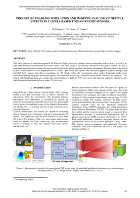
- Druml, N. et al. (2015). REAL3™ 3D Image Sensor. Infineon Technologies.
- Jarabo, A., et al. (2017). A Framework for Transient Rendering. ACM Computing Surveys.
- Lange, R. (2000). 3D Time-of-Flight Distance Measurement with Custom Solid-State Image Sensors in CMOS/CCD-Technology. PhD Thesis, University of Siegen.
- Remondino, F., & Stoppa, D. (Eds.). (2013). TOF Range-Imaging Cameras. Springer.
- Schwarte, R., et al. (1997). A New Electrooptical Mixing and Correlating Sensor: Facilities and Applications of the Photonic Mixer Device (PMD). Proc. SPIE.
- Zhu, J.-Y., et al. (2017). Unpaired Image-to-Image Translation using Cycle-Consistent Adversarial Networks. IEEE International Conference on Computer Vision (ICCV). (CycleGAN reference for synthetic data generation).
- NVIDIA OptiX Ray Tracing Engine. (n.d.). Retrieved from developer.nvidia.com/optix.